I recently found myself driving from Wellington to Auckland to save money and carbon for conference travel. For anyone not from NZ, it's a pretty long way. And so, on the way back I had lots of time to think, and somewhere around Hamilton I decided it would be a GREAT idea to scrape the tweets from the conference hashtag, and make a word cloud.
Sadly, I didn't know how to scrape tweets, and my text analysis skills are pretty basic. But, I had my laptop and nearly an hour to kill, and my co-pilot was driving. Bring it on!
Step 1 was finding out how to scrape tweets. It turns out to be pretty easy, especially if someone else has already written the code (thank you, vickyqian!) Click here for a python script that scrapes a hashtag of your choice (or any search term) and writes the results to a CSV file. It worked first time for me. I tried to incorporate it into my Rmarkdown below, but it's not working for me at the moment. If I ever work out how to use python through R, I'll update it!
To get the script working, you'll need tweepy, as well as csv and pandas. You'll also need to get a consumer API token and secret, and and access token and secret, from Twitter's Developer platform. I'll admit I had basically no idea what I was doing here - it's easy to set up an account (and free), and you'll need to create an app in order to get the tokens. I did this with the help of my BFF, Google.
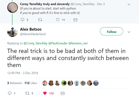
Note: I have since discovered that you can do all of this in R through the 'rtweet' package. But hey, I need to improve my python, and my coding philosophy is pretty well summed up by
this tweet.
First attempt using tm
Next you just need to read in the resulting CSV file to R, tidy it, turn the raw tweets into a word frequency table, and make a wordcloud. I initially did this using the R packages tm and wordcloud2. I guess you could also do this in python, but please refer to figure 1 above.
I’ve since improved this script but I’ll give you both versions so you can see some alternative ways of doing this.
dat<-read.csv("nzes.csv") # read in CSV outputted from python script

dat2<-data.frame(dat[,2]) # drop the date column, we don't need it

library(tm)
library(wordcloud2)

# loop through each tweet (row), tidying it by setting to lower case, remove punctuation, numbers and
# whitespace. Then look at resulting list and manually remove common joining words, names, unwanted words.

for (i in 1:nrow(dat2)){
  a<-tolower(dat2[i,1])
  b<-removePunctuation(a)
  c<-removeNumbers(b)
  d<-stripWhitespace(c)
  e<-removeWords(d, c("rt", "nzes", "the", "and", "for",
                      "with", "about", "from", "how",
                      "are", "that", "our", "loraxcate",
                      "jennypannell", "adzebill", "around",
                      "this", "amybmartian"))
  dat2$new[i]<-e

}
Next, you need to turn the strings of tweets into a data frame or matrix of individual words and their frequencies:
temp<-VectorSource(dat2$new)
newdat<-VCorpus(temp)

dtm <- TermDocumentMatrix(newdat)
m <- as.matrix(dtm)
v <- sort(rowSums(m),decreasing=TRUE)
d <- data.frame(word = names(v),freq=v)
head(d, 10)
## word freq
## plant plant 99
## nzecology nzecology 64
## conservation conservation 60
## ecology ecology 60
## talk talk 57
## phd phd 55
## can can 54
## love love 54
## come come 53
## potential potential 48And finally, turn that data frame into a wordcloud using the ‘wordcloud2’ library
wordcloud2(d)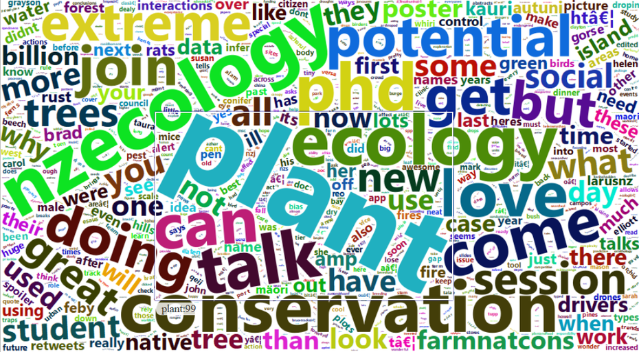
Pretty neat! I tweeted the result at the organizers when I was done (original tweet here), but it was still far from
perfect. I then found this wonderful blog that talked me through a much tidier and better method.
Second attempt using tidytext
dat<-read.csv("nzes.csv", stringsAsFactors=FALSE, header=FALSE)
# strings as factors is vital to stop R from messing this whole thing up!

library(tm)
library(tidytext)
library(dplyr)
library(stringr)
library(wordcloud2)

dat2<-data_frame(txt=dat$V2) # remove the date column
As before, we need to tidy the data up, but this time I did a more thorough job:
# remove words beginning with @ at this point before it gets stripped by unnest_tokens
# also for specific plural instances
dat2$txt<-gsub("@\\w+ *", "", dat2$txt) # remove twitter handles
dat2$txt<-gsub("1080", "ten-eighty", dat2$txt) # specific number I'd like to keep
dat2$txt<-gsub("nz", "newzealand", dat2$txt) # specific 2 letter word I'd like to keep
dat2$txt<-removeNumbers(dat2$txt) # remove numbers & punctuation
dat2$txt<-removePunctuation(dat2$txt)

# deal with duplicate words & some more specific words to keep
dat2$txt<-gsub("seedlings", "seedling", dat2$txt)
dat2$txt<-gsub("spp", "species", dat2$txt)
dat2$txt<-gsub("ecosystems", "ecosystem", dat2$txt)
dat2$txt<-gsub("everyones", "everyone", dat2$txt)
dat2$txt<-gsub("papers", "paper", dat2$txt)
dat2$txt<-gsub("peoples", "people", dat2$txt)
dat2$txt<-gsub("te reo", "tereo", dat2$txt) # make sure to keep as 1 word
dat2$txt<-gsub("\\breo\\b", "tereo", dat2$txt)
dat2$txt<-gsub("\\bte\\b", "tereo", dat2$txt)

# use the unnest_tokens function in tidytext to make the word frequency table
# make into data frame with 1 row per word = 13339 words
datTable <- dat2 %>%
  unnest_tokens(word, txt)
OK, so I’m immediately sold by tidytext. Turns out it’s also brilliant at removing unwanted words:
#remove stop words - aka typically very common words such as "the", "of" etc
# now 7770 words
data(stop_words)
datTable <- datTable %>%
  anti_join(stop_words)

#add word count to table
datTable <- datTable %>%
  count(word, sort = TRUE)
Looking good, but there are still some strange characters in there along with names, etc. Plus it’s unmanageably big, so let’s remove all words that occur less than 3 times.
#Remove other nonsense words, names, etc
# Also remove all with count < 3
datTable <-datTable %>%
  mutate(word = stripWhitespace(word)) %>%
  mutate(word = gsub(".*â.*", "", word)) %>%
  mutate(word = gsub(".*s.*", "", word))%>%
  mutate(word = gsub(".*ä.*", "", word))%>%
  mutate(word = gsub(".*ã.*", "", word))%>%
  mutate(word = gsub(".*ð.*", "", word))%>%
  mutate(word = gsub(".*ÿ.*", "", word))%>%
  mutate(word = gsub("\\b\\w{1,2}\\b","",word))%>%
  filter(!word %in% c('rt', 'https', 'tco', 'nzes', 'feby',"its", 'amp', 'psfcqudknr', 'ori', 'sullivan',
                      'carol', 'elliott', 'gt', 'helen', 'john', 'reo', 'richelle', 'suryaningrum',
                      'susan', '', 'bn', 'kristine', 'febyana', 'brad', 'griffiths', 'graeme',
                      'grayson', 'greenfirebreaks', 'kristine', 'dr', 'greatâ', 'james',
                      'nzj', 'annemieke', 'ayhrtyp', 'azharul','esaus', 'gaskett', 'ha', 'hendriks', 'ivan',
                      'mason', 'md', 'nzs', 'ough', 'sarah', 'tom', 'zealand', 'th', 'am', 'aoc',  'azhar',
                      'clayton', 'dawes', 'dont', 'herses', 'howell', 'jadewafuw', 'newzealandes', 'olivia',
                      'pattrmerns', 'tupp', 'bskmsdnih', 'connolly', 'elrhfakqb', 'eqsgewpt', 'herse',
                      'julia', 'kmubjomcm', 'lauren', 'muylaert', 'nqpfdgpdd', 'patters', 'renata', 'simon',
                      'stepts', 'thvdsmraii', 'walker', 'xkhombbhq', 'waller', 'xkhombbhq', 'xclhuxi',
                      'hgihzpgt', 'abigail', 'newzealands', 'newzealandj', 'ill', 'didnt', 'httpstcopsfcqudknr'
                      )) %>%
  subset(., n>2)
Finally, I tried to improve upon my original word cloud by changing the colours. I also tried to add a mask as per the littlemissdata blog post, but it didn’t work for me. It seems others have had similar issues and there’s a bug in the wordcloud2 package. I also spent about an hour playing with the ‘ggwordcloud’ package, but I wasn’t a fan. I also still coudln’t get the mask to work. If anyone has successfully done this, please let me know!
#Create Palette - I used Canva.com for inspiration
greenPalette <- c("#3D550C", "#81B622", "#ECF87F", "#59981A", "#D4D6CF")

wordcloud2(datTable, color=rep_len(greenPalette, nrow(datTable)))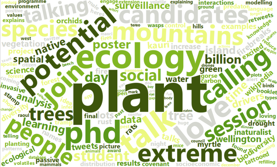
In the end, I gave up and exported the data table to a CSV and used a free website to make the finished version, shaped like the iconic kiwi (it was for the NZ ecological society, after all). It feels a bit like cheating though, so if you've worked with word clouds, please let me know your method of choice!
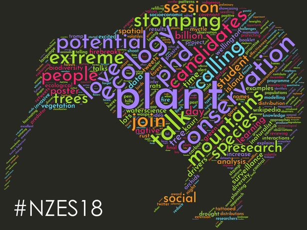
Here's the finished product! Much improved since the first version, but getting from zero to a rough version took about an hour. I'll try to use my more of my travel time for mini projects in future!

Write a comment